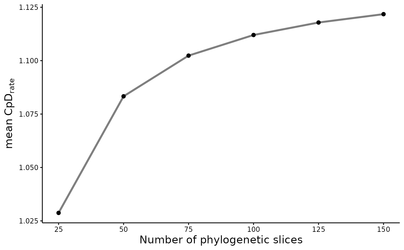
Make a plot of the sensitivity analysis evaluated under cumulative phylogenetic rate functions

This function generates a plot of the sensitivity analysis calculated for a given cumulative phylogenetic rate (CpR) assessed through the CpR_sensitivity() function.

Usage

CpR_sensitivity_plot(sst_output, rate = NULL, stc = "mean")

Arguments

sst_output: data frame. The outputted data frame from the CpR_sensitivity() function.
rate: character string. The desired phylogenetic index rate to display. It can be filled with "CpD", "CPE", "CpB", or "CpB_RW".
stc: character string. A statistical measure to summarize the phylogenetic rates and create the plot, which could be filled with "mean", "var", "median", "sd", "min", and "max". Default is "mean".

Value

The function returns a ggplot graph.

References

Users can use the CpR_sensitivity_plot() function for plotting sensitivity analysis outputs.

Author

Matheus Lima de Araujo matheusaraujolima@live.com

Examples

# Generate a random tree
tree <- ape::rcoal(20)

# Create a presence-absence matrix
mat <- matrix(sample(c(1,0), 20*10, replace = TRUE), ncol = 20, nrow = 10)
colnames(mat) <- tree$tip.label

# Calculate the CpD for 100 tree slices
CpD(tree, n = 100, mat = mat)
#> > The 100 number of pieces inputted equals to intervals of 0.0180875415751787 million of years.
#>         CpD       PD      pDO
#> 1  1.139800 5.597501 2.628296
#> 2  1.092982 5.323702 2.740881
#> 3  1.126685 5.539343 2.658890
#> 4  1.013498 4.914616 2.955833
#> 5  1.175538 5.771475 2.548393
#> 6  1.029199 4.982034 2.910742
#> 7  1.175538 5.771475 2.548393
#> 8  1.098712 5.410340 2.726586
#> 9  1.175538 5.771475 2.548393
#> 10 1.138231 5.587802 2.631921

# Create a vector of number of slices
vec <- c(25, 50, 75, 100, 125, 150)

# Calculate the sensitivity of the CpD
Sens_out <- CpR_sensitivity(tree, vec, mat, rate = "CpD", samp = 5)
#> Warning: Removing the species in presence abscence matrix without any occurrence
#> Warning: Removing tips from phylogeny that are absent on species matrix
#> > The 25 number of pieces inputted equals to intervals of 0.0723501663007148 million of years.
#> Warning: Removing the species in presence abscence matrix without any occurrence
#> Warning: Removing tips from phylogeny that are absent on species matrix
#> > The 50 number of pieces inputted equals to intervals of 0.0361750831503574 million of years.
#> Warning: Removing the species in presence abscence matrix without any occurrence
#> Warning: Removing tips from phylogeny that are absent on species matrix
#> > The 75 number of pieces inputted equals to intervals of 0.0241167221002383 million of years.
#> Warning: Removing the species in presence abscence matrix without any occurrence
#> Warning: Removing tips from phylogeny that are absent on species matrix
#> > The 100 number of pieces inputted equals to intervals of 0.0180875415751787 million of years.
#> Warning: Removing the species in presence abscence matrix without any occurrence
#> Warning: Removing tips from phylogeny that are absent on species matrix
#> > The 125 number of pieces inputted equals to intervals of 0.014470033260143 million of years.
#> Warning: Removing the species in presence abscence matrix without any occurrence
#> Warning: Removing tips from phylogeny that are absent on species matrix
#> > The 150 number of pieces inputted equals to intervals of 0.0120583610501191 million of years.

# Plot the sensitity analysis
CpR_sensitivity_plot(Sens_out, rate = "CpD", stc = "mean")