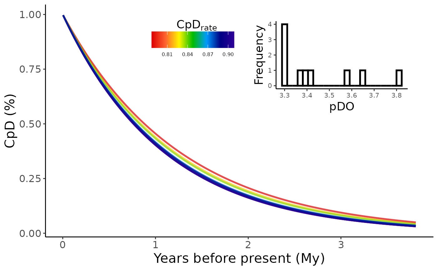
Make a line graph or a grid map of estimated rates of accumulation of a given phylogenetic index.

This function creates a line graph, or a grid map, depicting the estimated rates of accumulation of a given phylogenetic index (e.g., phylogenetic diversity, endemism, etc.), obtained from functions such as CpD(), CpE(), CpB(), or CpB_RW().

Usage

CpR_graph(data, rate = NULL, map = NULL, pal = NULL, qtl = FALSE)

Arguments

data

data frame. The outputted data frame from a CpR-rate function.

rate

character string. The desired cumulative phylogenetic rate to plot, which can be phylogenetic diversity (CpD), phylogenetic endemism (CpE), phylogenetic B-diversity (CpB), or phylogenetic B-diversity range-weighted (CpB_RW). Default is NULL, but must be filled with "CpD", "CPE", "CpB", or "CpB_RW".

map

spatial data. A grid map containing the assemblages at which the phylogenetic rates were assessed. Default is NULL.

pal

character vector. A vector containing a color palette. If none provided, a default color palette will be used.

qtl

boolean. Should the color palette be displayed according to CpR-rates quantiles? It can be either TRUE or FALSE. Default is FALSE.

Value

The function returns a ggplot graph.

References

See the tutorial on how to use this function on our website.

See also

Other cumulative phylogenetic rate analysis: CpD(), CpE(), CpB(), CpB_RW(), CpR_sensitivity() Other plotting: CpR_sensitivity_plot().

Author

Matheus Lima de Araujo matheusaraujolima@live.com

Examples

# Generate a random tree
tree <- ape::rcoal(20)

# Create a presence-absence matrix
mat <- matrix(sample(c(1,0), 20*10, replace = TRUE), ncol = 20, nrow = 10)
colnames(mat) <- tree$tip.label

# Calculate the CpD for 100 tree slices
CpD_DF <- CpD(tree, n = 100, mat = mat)
#> > The 100 number of pieces inputted equals to intervals of 0.0232907007630734 million of years.

# Plot it using the CpR_graph
CpR_graph(CpD_DF, rate = "CpD")